On March 30, 2020, the ACM announced that its digital library would be open access for three months. During that time, every conference paper, journal article and book chapter published by the ACM was free to the general public. They didn’t even require a login. The reason to open the digital library was a good one: most people who use it get access through where they work, either in industry or academia. Because of the global pandemic, most people who use it are now working at home, outside of the network which allows them access.

I hoped it would remain open. I shared URLs to papers on the Digital Library on forums, in emails and even in source repos knowing everyone could access the papers at the moment, and hoping that would continue. I even let myself think it was likely that those making the decisions at the ACM would see that this free access had become a public good. I was wrong. On schedule, the ACM Digital Library closed again on June 30, 2020.

It should have remained open. First, because the global pandemic is not over, and few people who read computer science research papers are back at work. Most people who work in the software industry are still at home, and there is still uncertainty about what will happen in American colleges and universities in the next school year.

But more importantly, the ACM Digital Library should have remained open because the most comprehensive repository of computer science research should be freely available to all.

What is the ACM? What is the Digital Library?

The Association for Computing Machinery, or ACM, is a non-profit professional organization for the field of computing. Its stated mission is to support “educators, researchers and professionals” who work in all forms of computing. In practice, I believe the members are primarily computer science educators and researchers and the efforts of the ACM reflect that.

One of the most important functions of the ACM are its conferences and journals. Researchers in academia and industry publish their work through peer-reviewed conference proceedings and journals. For any given field in computer science, there is usually an ACM conference or journal which is one of the top venues to publish in for that field.

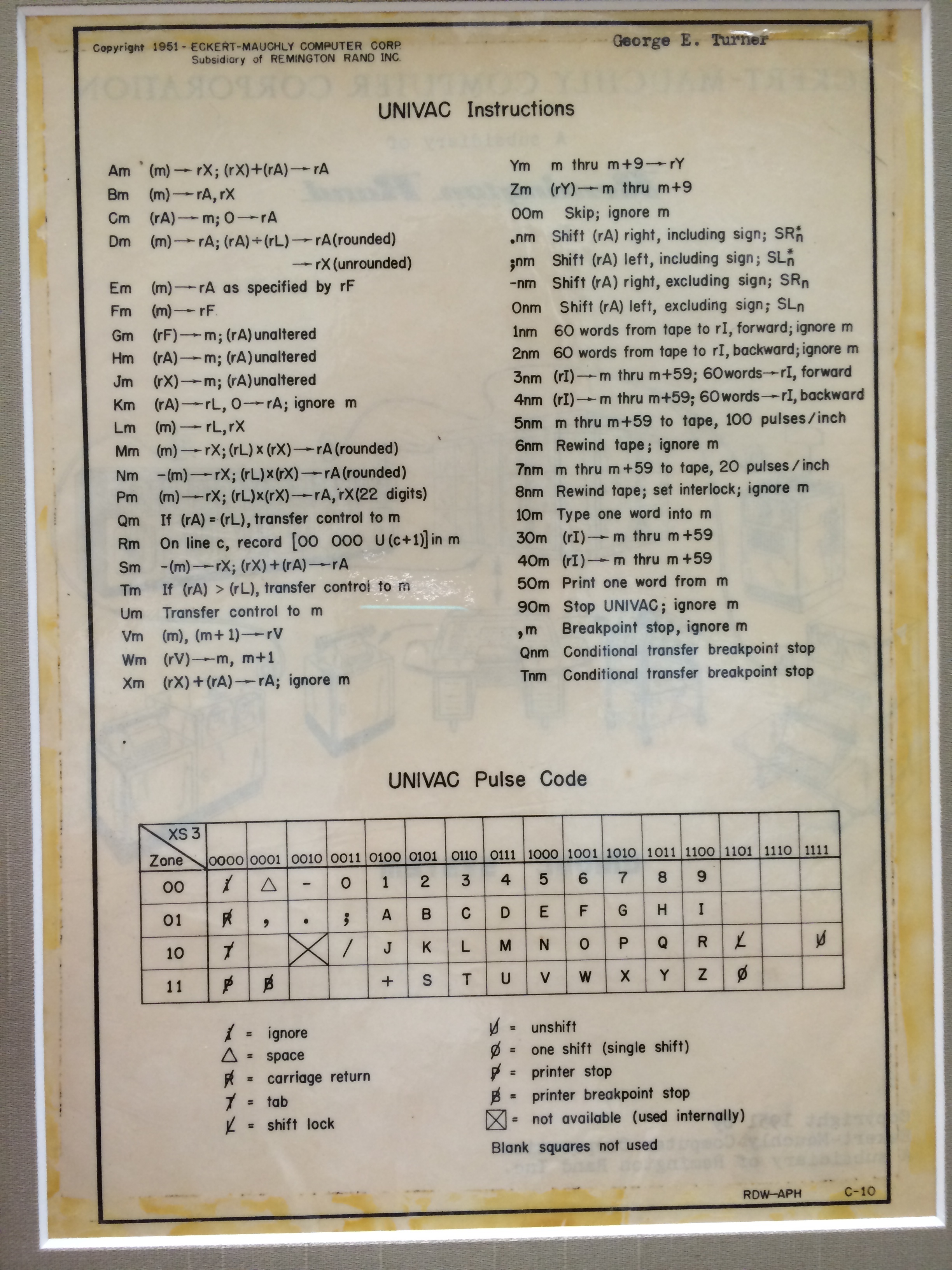
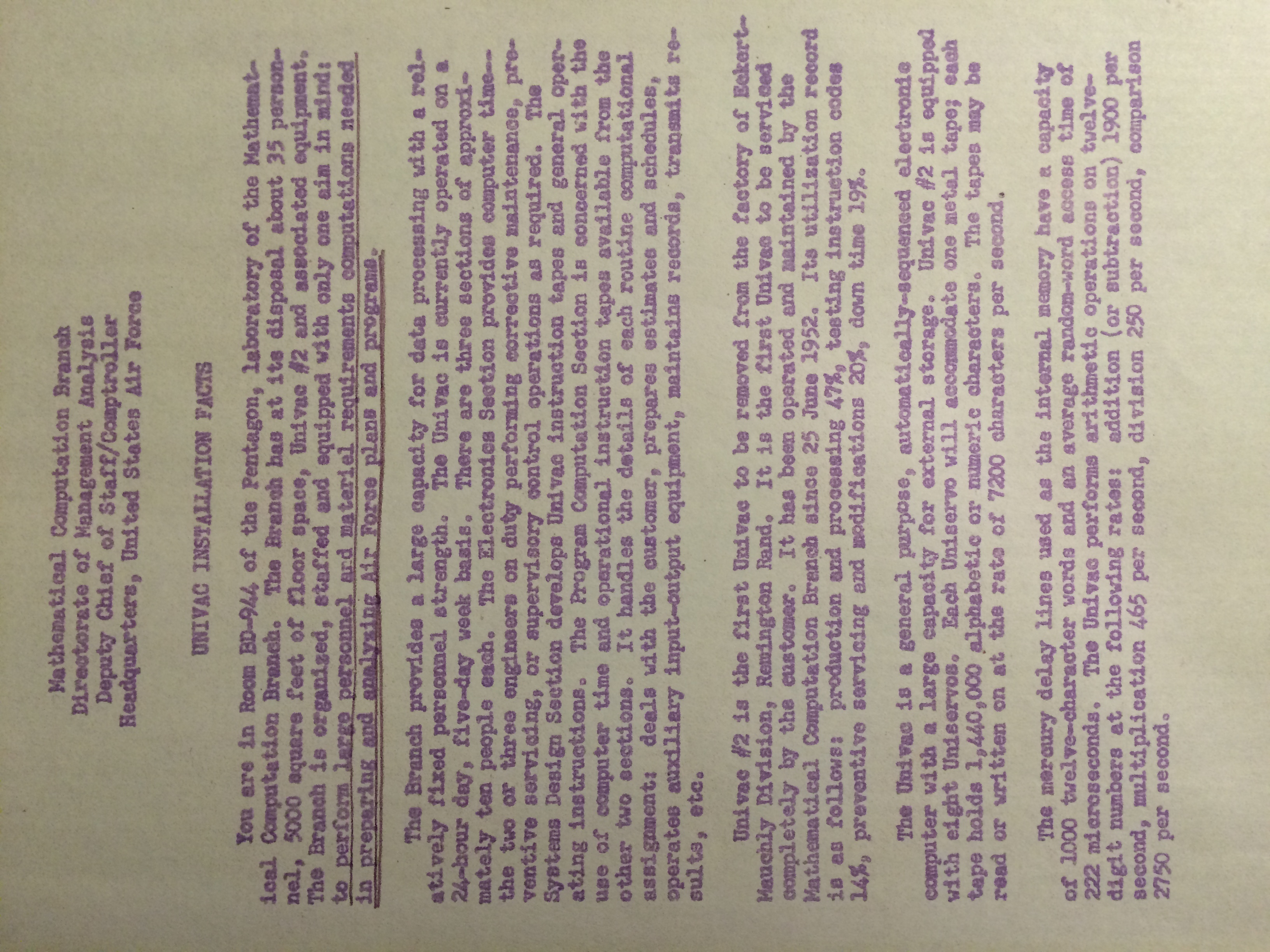
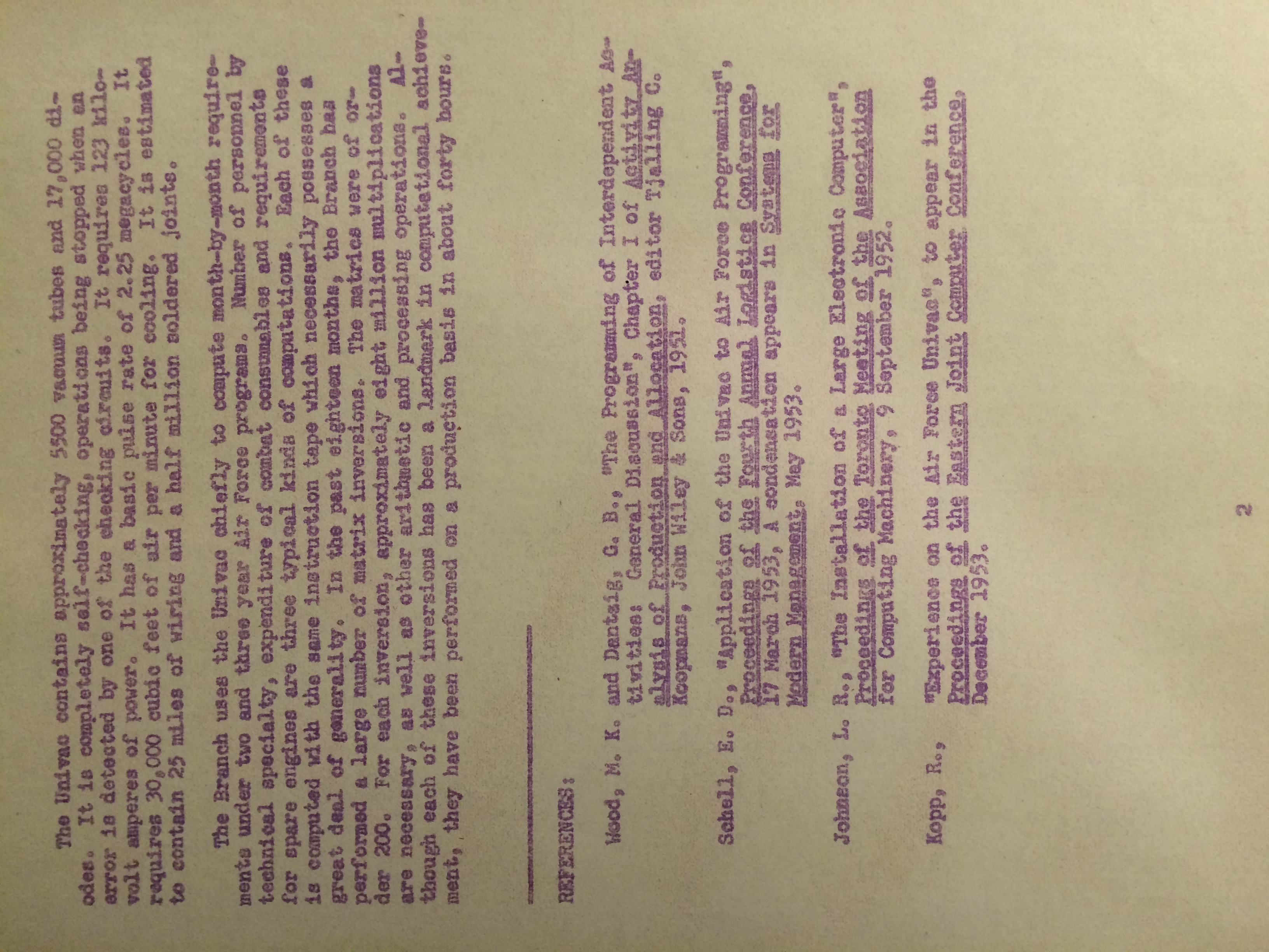
The Digital Library is the online repository for all of this research. It has papers published this month all the way back to the beginning of the field of computing in the early 1950s. It is, as far as I know, the most comprehensive single source of computer science research in the world.

What the ACM is not

The ACM is not a for-profit publisher. They are, as said above, a non-profit professional organization. This fact distinguishes them from for-profit publishers like Elsevier. There is a long-standing effort by many in the scientific community to boycott Elsevier and move to open access publications. This boycott has resulted in many organizations ending contracts including Dutch, German and Swedish universities, the University of California system and MIT.

For Elsevier, this fight for open access is existential. They exist to make a profit on scientific publishing. If Elsevier can’t charge for access to the papers it has published, it has no business model and it will cease to exist. The ACM exists to serve the field of computing and society itself. The purpose of the ACM is laid out clearly in Article 2 of its constitution:

The Association is an international scientific and educational organization dedicated to advancing the art, science, engineering, and application of information technology, serving both professional and public interests by fostering the open interchange of information and by promoting the highest professional and ethical standards.

Opening the ACM Digital Library supports every part of that sentence.

My impression is that practitioners are underrepresented in the ACM. These are the professional software developers, product managers and system administrators who do the majority of the professional computing work in our industry. The ACM has on the order of 100,000 members, which is surely a small fraction of the total computing professionals in the world.

When then-president Vint Cerf asked why so many professionals are not members, the closed Digital Library was one of the top answers. Professional organizations exist to serve the profession and the professionals in it—even non-members. The Digital Library should not be a membership perk. It should be the public resource that inspires professionals to become members.

Can’t we get the papers elsewhere?

The moment you write something, you own its copyright. In order for the ACM to publish a paper, we have to transfer copyright. Per that agreement, authors retain the right to publish the paper on their home page (which I do). The institutions the authors work at and the agencies that funded the work are also allowed to publish the paper.

Savvy readers without access to the Digital Library know this fact. Most recent papers can be found by simply Googling its title. Occasionally, finding a free copy of a recent paper requires tracking it down directly from authors’ homepages or institutional publication lists.

If most recent papers are available elsewhere, why all the fuss? There are four reasons:

1. Not all recent papers are posted by their authors or institutions. Authors don’t always update their home pages and institutions don’t always post papers. Some authors don’t even have a home page.
2. Older papers, from before authors routinely had a home page, are not freely available anywhere.
3. The Digital Library URL for a paper should be the canonical online home for that paper. If the author does not have a home page or the institution they work for ceases to exist, that URL will always be valid. But people are less likely to share that URL if not everyone can access it. Rather, they will point to the versions scattered throughout the internet.
4. The Digital Library itself is valuable: it is a well-designed network of papers, authors, conferences and journals. If you find an interesting paper, you can then easily look at the other papers published in the same conference. Or other papers published by the same author.

I know I’m being unfair

Rationally, three months of open access is better than zero, so the current situation is better than before. Yet, instead of giving the ACM credit for those three months, I’m asking for more. I acknowledge that is unfair. I also acknowledge that the ACM has stated that their eventual goal is general open access. They have several efforts towards this goal: ACM conferences can choose to grant open access to their latest proceedings; authors can pay a fixed fee for their paper to be open; and they established entire journals where all articles must pay the fixed fee to be open.

This is progress, and we must grant credit for incremental improvements. But I fear the ACM is still being too conservative: these efforts are ad-hoc, do not apply to historical papers and do not seem to make open access the primary goal.

I freely admit that I do not know what a sustainable model would look like. But I do know it is possible. While they are smaller in scope, there are major computer science conferences and journals that are completely open access, such as USENIX and VLDB.

I am a member of the ACM, and I intend to be a member for the rest of my life. I criticize it not because it is bad, but because I believe it is good. I just want it to be better.

I contribute posts over at StreamsDev, which is the developer-run community for the product I do research and development for, IBM Streams. These posts all involve SPL (Streams Processing Language), the programming language for developing applications on Streams.

We have an academic paper which covers the design of SPL. In brief, SPL is designed to be a programming language for distributed stream computing. The primary abstractions are operators, tuples and streams. Operators are the primary actors in the language; they receive tuples, perform computations on them, and potentially emit tuples which represent the result of that computation. Operators send and receive these tuples over streams, which are the only way they can communicate. Because operators can only communicate with each other over streams, the programming model is similar to functional languages, where functions can only “communicate” by accepting and returning values. Because the programming model of SPL forces operators to be fully isolated from each other, acting on on their explicit inputs and outputs, the language is amenable to various kinds of parallelization.

The first set of posts are brief programming tutorials, introducing some advanced techniques in SPL:

• Wrapping Custom operators in Composites: Custom operators in SPL are a way to introduce new operator logic. Composite operators are a way to represent a streaming sub-graph (a collection of operators that communicate with each other) as a single operator. Invoking a single custom operator inside of a composite is similar to assigning an anonymous function to a variable in functional languages.
• Genericity & Composites: In SPL, composite operators are to primitive operators as functions are to expressions in general purpose languages. Specifically, a composite operator is a reusable grouping of multiple operators with well-defined inputs and outputs so that it can be used as a single operator elsewhere in an application. This post explores one of the primary benefits of composite operators, which is that they can be generic with respect to the types they use and operate on.
• Operator Genericity: Genericity in SPL extends to operators themselves, and composite operators can actually accept other operators as parameters. This capability makes composite operators higher order.
• General Operator Parameters in UDP Regions: A specific technique for using several orthogonal features in SPL (custom state on operator invocations, operator parallelization and runtime specification of parameters) to use operators in parallel that were not designed for parallelism.

One of the primary reasons to write an application in SPL is to process a large amount of data quickly. The design of SPL allows programmers to first write an application focusing on functionality, and only consider performance after the application is correct. SPL exposes controls that allow programmers to tune their application for the underlying hardware. The post Optimizing Streams Applications presents the slides from a presentation I gave which teaches how the abstractions in SPL map to the underlying hardware in a cluster. It presents the application-level controls that SPL exposes, shows how to use them, and walks through improving the performance of an example application.

Finally, two posts which involved some actual research, in that they involved a significant amount of experimental evaluation:

• Parallelized File Processing with the Parse Operator: Any real streaming application is going to have to read data from an external source, as well as parse that data from the external format to an internal representation. Sometimes, the parsing is more expensive than the reading, and in such cases, we can use parallelism to improve throughput. This post motivates why parsing may be more expensive, and walks through developing a pattern programmers can use in such situations.
• The ElasticLoadBalance Operator: Elasticity, in this context, is dynamically adjusting the level of parallelism to maximize throughput. I adapted prior research work on elasticity into a reusable operator that can be used in the product. In this post, I explain how the elasticity algorithm works, why I had to change it from our previously published work, how to use the new operator, and experimental results demonstrating its effectiveness.

Pictured below is my grandfather’s cheat sheet for the UNIVAC I. He typed his name, George Eugene Turner, in the upper right. The copyright, in the upper left, reads 1951. (Click for a larger image.)

The ghost image is the reverse side of the sheet, which is the cover to the manual. The UNIVAC I was the first digital, electronic, general purpose computer built it one location, and moved to another location for operation. (The first digital, electronic, general purpose computer was the ENIAC. For an excellent history of it, read ENIAC: The Triumphs and Tragedies of the World’s First Computer by Scott McCartney.)

My grandfather was one of the first people to use it—that my grandfather used some of the first computers has been a part of family lore as long as I can remember. What was uncertain to me, however, was which UNIVAC he worked with. The first one? It appears so.

In the the retrospective Coming to Grips with the UNIVAC by Lyle Johnson, he writes:

Once the Census Univac had passed its tests, Remington Rand management naturally expected prompt acceptance of the second system. The factory raced to meet its target date of mid-November. Schell and I were observers when testing started on 13 November. The CPU, as well as our two Unitypers (offline keyboard-to-tape units) and two Uniprinters (offline tape-fed typewriter printers), were soon deemed acceptable. But our Uniservos—the eight magnetic tape devices connected to the CPU, were not. We returned for testing on 27 November and stayed over, again to learn that NBS was holding up delivery.

Meanwhile, Schell made a deal with Census for use of its computer over the New Year weekend. Three of our programmers—Natalie Coplan, Harold Fisher, and George Turner agreed to use the time for program debugging. Schell and I went along to reassure Census management, provide moral support, and gain familiarity with the Univac. We were there 29-31 December 1951 and 1 January 1952. This was my opportunity to examine devices, mount reels of metal tape, decode data indicated by the many little neon lamps, watch read/write error- recovery processes, and ask questions of Eckert-Mauchly engineers during maintenance. All told, it was an exciting weekend.

The first UNIVAC I went to Census, but it was not actually the first one shipped. The first shipped UNIVAC I went to the Air Force. However, it appears that my grandfather also programmed on the Air Force’s UNIVAC. Picture below is a document we have from the Mathematical Computation Branch of the United States Air Force. (Click for a larger image.)

The document says:

You are in Room BD-944 of the Pentagon, laboratory of the Mathematical Computation Branch. The Branch has at its disposal about 35 personnel, 5000 square feet of floor space, Univac #2 and associated equipment. The Branch is organized, staffed and equipped with only one aim in mind: to perform large personnel and material requirements computations needed in preparing and analyzing Air Force plans and programs.

The Branch provides a large capacity for data processing with a relatively fixed personnel strength. The Univac is currently operated on a 24-hour, five-day week basis. There are three sections of approximately ten people each. The Electronics Section provides computer time—the two or three engineers on duty performing corrective maintenance, preventive servicing, or supervisory control operations as required. The Systems Design Section develops Univac instruction tapes and general operating instructions. The Program Computation Section is concerned with the use of computer time and operational instruction tapes available from the other two sections. It handles the details of each routine computational assignment; deals with the customer, prepares estimates and schedules, operates auxiliary input-output equipment, maintains records, transmits results, etc.

Univac #2 is the first Univac to be removed from the factory of Eckert-Mauchly Division, Remington Rand. It is the first Univac to be serviced completely by the customer. It has been operated and maintained by the Mathematical Computation Branch since 25 June 1952. Its utilization record is as follows: production and processing 47%, testing instruction codes 14%, preventative servicing and modifications 20%, down time 19%.

The Univac is a general purpose, automatically-sequenced electronic computer with a large capacity for external storage. Univac #2 is equipped with eight Uniservos. Each Uniservo will accommodate on metal tape; each tape holds 1,440,000 alphabetic or numeric characters. The tapes may be read or written on at the rate of 7200 characters per second.

The mercury delay lines used as the internal memory have a capacity of 1000 twelve-character words and an average random-word access time of 222 microseconds. The Univac performs arithmetic operations on twelve-digit numbers at the following rates: addition (or subtraction) 1900 per second, multiplication 465 per second, division 250 per second, comparison 2750 per second.

The Univac contains approximately 5500 vacuum tubes and 17,000 diodes. It is completely self-checking, operations being stopped when an error is detected by one of the checking circuits. It requires 123 kilovolt amperes of power. It has a basic pulse rate of 2.25 megacycles. It requires 30,000 cubic feet of air per minute for cooling. It is estimated to contain 25 miles of wiring and a half million soldered joints.

The Branch uses the Univac chiefly to compute month-by-month requirements under two and three year Air Force programs. Number of personnel by technical specialty, expenditure of combat consumables and requirements for spare engines are three typical kinds of computations. Each of these is computed with the same instruction tape which necessarily possesses a great deal of generality. In the past eighteen months, the Branch has performed a large number of matrix inversions. The matrices were of order 200. For each inversion, approximately eight million multiplications are necessary, as well as other arithmetic and processing operations. Although each of these inversions has been a landmark in computational achievement, they have been performed on a production basis in about forty hours.

A few observations:

• The document says “Univac #2”, but it means UNIVAC I, #2. The UNIVAC I was not called such until the UNIVAC II.
• The character reading and writing rate (7200 characters per second) is greater than the fastest computation rate (2750 comparisons per second). Depending on the number of characters required to represent a number, input and output for some data could be faster than its processing. This relationship would not hold as computers advanced. In modern systems, processing has outstripped reading and writing to the point that we frequently trade significant processing time for a little less reading and writing. Two examples are compressing data before writing, and sophisticated paging algorithms.
• The relative cost of division to addition is similar to what it is today.
• Even in the beginning, we needed to cool our systems.
• A matrix inversion of 200 elements was considered a “landmark in computational achievement”.

My grandfather is also credited as a UNIVAC I Pioneer, acknowledged in the 1960 Census, and is credited as the Chief Programmer, Survey of Components of Change and Residential Finance for it.

By the modern definition of the word, my grandfather was one of the first programmers.

Thanks to Dan Gackle for reviewing a draft of this essay.

A decade ago, I was a new graduate student at William and Mary taking a course called “Linux Kernel Internals.” For this course, we all presented a walk-through of a particular part of the kernel. I had the boot process, and I created the slides Booting: From Power Up to Login Prompt.

The slides can be read on their own. This kind of a code walk-through reinforces a mantra I repeat when it comes to understanding computer systems: It’s all just code. We can always understand a computer system by systematically reading the code.

A fundamental tenet of modern biology is that life happened once. In principle, we can trace the lineage of everything alive today back to that occurrence. And, as a consequence, everything alive is related.

We can infer how related everything is by comparing the genomes of different species. Because the genomes for humans and chimps are “less different” than the genomes for humans and gorillas, we conclude that humans and chimps are “more related.” In this context, “more related” means that as we go backward in time, we encounter the most recent common ancestor between humans and chimps before we encounter the most recent common ancestor between humans and gorillas.

The generalization of this concept is the phylogenetic tree. Given a set of genomes, we can visualize the relatedness of the set of species by placing “more related” species fewer hops away in the tree from “less related” species. The convergence point for different species in the tree is their most recent common ancestor. The root of the phylogenetic tree is that first occurrence of life, the ancestor to everything alive.

Let’s create an analogy where biological species map to compilers, and individual organisms within a species map to programs created by a particular compiler. We’ll call this a phylobinary tree as “binaries” is common shorthand to mean “compiled, executable programs.” (This is not to be confused with the binary tree data structure.)

The full phylobinary tree would contain all existing compilers as nodes. If a compiler is an internal node in the tree, it means that that compiler was used to create another compiler—compilers are, after all, just programs like any other. For example, the gc compiler for Go is implemented in C. This means that every compilation of gc will be a child of the C compiler that created it. Note that this is a mechanical relationship, as opposed to a conceptual one. There are many attempts to show conceptual relationships between programming languages, where a parent-child relationship means that ideas in the parent language influenced similar ideas in the child language. Instead, phylobinary trees are about actual, compiled programs. The aforementioned gc compiler will have many entries in the phylobinary tree: one for each distinct binary.

“Distinct binary” does not mean that we count copies of a binary multiple times; copies are indistinguishable. If two binaries are identical, they map to the same place in the phylobinary tree. But, each compiler version, for each different architecture, for each different operating system, will have distinct entries in the phylobinary tree.

We, obviously, have not done the work necessary to construct the full phylobinary tree. (And I am deliberately saying “the” full phylobinary tree, not “a” full phylobinary tree; whatever it looks like, there is only one full phylobinary tree at any given time.) However, we can still reason about its properties.

Roots and Forests

First, unlike the full phylogenetic tree, the full phylobinary tree will not have a single root. A root in the full phylobinary tree is a compiler that was not compiled by another compiler; it was created by hand in assembler. (We could extend the definition of our phylobinary tree to include assemblers, but the tree would be much messier, and I don’t think we would gain any extra insights.) Certainly, many compilers were created by hand—decades ago, it was a necessity. And it is very likely that many programs that exist today can be traced back to distinct compilers that were created by hand. An interesting question, then, is how many roots does the full phylobinary tree for this moment in time contain? We can’t answer this question without constructing the full tree.

In fact, if we look at all programs in current use now, the “tree” will actually be a forest with many disjoint trees. Any program that is not a compiler and written directly in assembly will be a completely disjoint node, with no other connections. (Note that this is necessarily true by how we have constructed the tree: only compilers have children, so a non-compiler cannot have children.) And there will likely be many compiler trees with no connections to each other.

My intuition is that the largest trees will involve C compilers. But how many trees, disjoint nodes, and total roots will the entire phylobinary graph have? I do not know. My guess is that the vast majority of running programs will exist on only a dozen or so trees, and trace back to about that many roots.

Tree Construction

While the easiest way to construct a phylobinary tree would be to keep records external to the binaries themselves of which compiler produced which executable program, it is not necessary. Genes are often compared to computer code. But we can go the other way, and analyze binaries in a similar way to how we analyze genes. The same compiler will tend to produce similar segments of code, even for different programs. In fact, the security community already takes advantage of this fact when analyzing malware. They commonly identify not just the source language from malware binaries, but even the particular compiler that produced it. When analyzing Duqu, Kaspersky Labs concluded that some of the code was C++, compiled by Microsoft Visual Studio C++. However, the majority of the binary code was something they had never seen before. They asked the community for help, and the conclusion was that it was an object-oriented dialect of C, also compiled by Microsoft Visual Studio C++.

If static analysis of binaries is akin to genetic analysis, then observing runtime behaviors of programs is akin to phenotype analysis. (A phenotype is some observable characteristic of an organism, which can be either a physical trait or a behavior.) There are academic projects which attempt to characterize the runtime behavior of malware, such as the BitBlaze project at UC Berekley. (I found their papers on extracting reusable sections of binaries, inferring protocols, and formal methods particularly interesting.)

I am unaware of anyone using a combination of these techniques to create phylobinary trees. I think it is clearly possible.

Cycles

The analysis by Kaspersky Labs raises another wrinkle: not all programs are the product of a single compiler. Many programs are linked together into a single binary from many different binary object files. Such binary object files can come from distinct compilers (and those compilers may even be for different languages). This wrinkle means that some programs will have multiple parents in the phylobinary tree.

Note that cycles are technically possible, so phylobinary trees are not strictly trees, but general graphs. Cycles can happen in one of two ways: multiple compilers producing a single compiler, and trickery. If compiler A produces compilers B₀ and B₁, and then both B₀ and B₁ are used to separately compile compiler C, then we have a cycle. This situation is unlikey, but not unrealistic.

The trickery way involves crafting programs to deliberately create cycles. Quines are programs that reproduce their own source code. But quines are about source code; we want a program that when it’s run, generates a copy of itself—not the source code, but an actual reproduction of the binary. I have only found one such example. That program, then, will be a cycle back onto itself. And, if 50 language quine-relays are possible, then it is likely that such quine binary relays are also possible. So we will not be limited to just single nodes that cycle back on themselves, but it should also be possible to have arbitrarily long chains that eventually end in a cycle.

It’s also interesting to note something that does not introduce new roots into trees: cross compilation. It’s tempting to assume that every disjoint tree in the phylobinary forest necessarily represents a single computer architecture, but that is not true. A compiler running on an x86 processor can still compile programs for an ARM processor. An x86 compiler can even compile an ARM compiler. No new roots are introduced by this process.

What might be true is that disjoint trees are very likely to contain programs from a single operating system. Note that in this binary-centric view of computing, source code similarity does not matter. If I port a compiler from one operating system to another, the resultant compiler will be a child of the compiler used to produce it, not the original compiler. That’s potentially confusing, so let’s be precise. Let’s assume I have a compiler for language Foo, which runs on Linux. The Foo compiler is implemented in C, and on Linux, I use a version of gcc. Now, I port the Foo compiler to Windows, and I use the Microsoft Visual Studio C++ compiler to compile my Foo compiler for Windows. My Foo compiler under Windows has no phylobinary relationship to the Foo compiler (or the gcc compiler) on Linux.

What is necessary to bridge such operating system disjoint trees in our phylobinary forest are cross operating system compiles. Such instances will be common with embedded devices, including iOS and Android. (And if you think that is interesting, you must look at what a Canadian Cross is.)

Conclusion

While I find the concept of phylobinary trees interesting, I’m not sure what use they are. Certainly some of the ideas are important for security, as previously mentioned—but they seem to get by just fine without a formalized framework. Perhaps it would be useful to be able to say to each other, “There is no known phylobinary root for this program” instead of “I do not know what compiler produced this program.” But perhaps not. The use could be less scientific, and more historical. For example, in a hundred years, will running programs be in a phylobinary tree with compilers that exist now? I think that’s likely. And I think it would be interesting if we actually had the information in a hundred years to answer that question.

Thanks to Ben DeVane, Dan Gackle and Will Slade for reviewing drafts of this essay.

To my surprise, some programmers consider using print statements instead of debuggers as a wholly inferior means of debugging. As I view the debugging process, they are complementary techniques. But the issue is not really “print statements” versus “debuggers.” It’s traces versus snapshots.

Traces provide a long term view over a small set of data, and snapshots show all of the data from a moment in time. Or, as a figure:

Traces

Most of my programming time is spent working on the runtimes for parallel systems. Whether it’s multithreaded memory allocation, automatic data transfers, or tracking messages in a distributed system, these all have one thing in common: they’re event based. The code I write is not the code driving the program; my code is servicing an application.

When I have bugs, they are typically algorithmic in nature. My code correctly implements my understanding of the problem, but my understanding is wrong. Rarely does a program actually crash. Segfaults are actually a relief, because diagnosing the problem will probably be easy: just fire up the debugger and find the null pointer or empty container.

Rather, most of the time, the end results of the program are wrong, and I need to figure out why. Doing so requires recording just enough of the execution of the program to be able to spot something that disagrees with my understanding of what should happen. In other words, I need a trace.

Typically, I start by instrumenting the most visible entries into the runtime system. For example, for a memory allocator, I’ll log every allocation and deallocation request. For an allocation, I’ll record the size and the memory address returned. For the deallocation, I’ll record the memory address being freed. Doing this provides me with a trace that is complete in time (it covers the whole execution of the program), but incomplete in program state (it is only for a select few values). But by having a trace, I can look forward and backward in time at my leisure, looking for aberrant behavior—say, the same memory address returned for two allocation requests without a deallocation in-between.

When tracking messages in a distributed system, I’ll log the receipt and submission of each message as they flow through the system. By looking at the traces for all of the processes in the system, I can construct the message flow and look for messages that are out of place.

I’m rarely lucky enough that these top-level traces provide enough information to find the bug. These traces are just the start, as they hint where to explore next. Do I need more data at my current level of instrumentation, or do I need to start instrumenting deeper parts of my algorithms? (Note that “instrumenting” is just a fancy way of saying “adding more print statements.”) In terms of my figure, I start with a narrow vertical slice of the program state, and selectively broaden its width as my understanding of the problem matures.

In situations like the above, a single snapshot of the entire program state is not going to show me what I need to know. A snapshot, as provided by a debugger, can tell me the entirety of the program’s state, but it cannot tell me how the program came to be in that state. I need history—lots of it. I could set breakpoints, observe the state, resume, wait for the next breakpoint, and then observe again. And sometimes, I do this. But doing this process thousands of times is not feasible—and good traces can easily reach into the hundreds-of thousands of events.

Snapshots

Of course, sometimes I still need snapshots. When a program crashes or hangs, I reach for a debugger. In those instances, I want to be able to inspect the entire system state at my leisure. Debuggers are essential for this, because it’s infeasible to log the entire system state; debuggers are interactive, and allow exploration of the system state much in the same way that traces allow exploration of algorithmic behavior over time.

Sometimes I’ll even reach for a debugger after spending a long time inspecting traces. If I can spot where things go wrong in a trace, but I’m already at the finest granularity of logging possible, then I start to suspect system issues like memory corruption. But in such a case, traces showed me where to look. I never would have been able to discover exactly where in my program to point the debugger without the trace. (I’m assuming, of course, that this is the kind of memory corruption that valgrind cannot find.)

Debuggers are for when I have started to question even the most fundamental of operations, and I need to observe exactly what is happening at a point in time. In fact, I can rely on traces because I already have a good idea of what the system is doing at all points of the program. When I use traces, what I question is not the system itself, but my algorithms that run on top of it. Once I start to suspect the system itself, I reach for the debugger.

A Mental Model

Whether using traces, snapshots or both, the purpose is to build a mental model of what your program is actually doing, because your current one is wrong. (If it wasn’t, you wouldn’t have a bug.) Knowing the entire state of your program during its entire time of execution is not realistic for interesting programs. So we investigate sections of the state-time space. And, in general, we want to look at slices that cover all of one of those dimensions. If I’m confident that a particular value is involved in an error, then I want to see all of those values, over all time—a vertical slice, a trace. If my view of the state-time space does not cover all time, then there’s always the possibility that the error is lurking somewhere in the times I did not cover. If I’m confident that an error occurs at a particular moment in time, then I want a horizontal slice, a snapshot, so I can observe all values across that moment.

If you ever find yourself producing single-line traces where you keep adding reported values, you don’t want a trace. You want a snapshot, and a debugger is the better tool. If you ever find yourself setting breakpoints in a debugger, writing down values, letting it run until the next breakpoint and again writing down values, then you don’t want a snapshot. You want a trace.

A surprisingly common sentiment among some programmers is that “computer science is math.” Certainly, computer science as a rigorous discipline emerged from mathematics. Now, we consider such foundational work to be theoretical computer science. For example, Alonzo Church’s lambda calculus and Alan Turing’s Turing machine provided a theoretical foundation for computation. At the time, the two self-identified as mathematicians, and were clearly doing mathematics. So if the foundations of computer science are math, how is it that computer science as a whole is not math?

Simply, computer science has grown well beyond its purely theoretical roots. We invented real computers, which are not theoretical devices. In doing so, we had to deal with the complicated and messy reality of designing, implementing, using and programming computers. Those areas of study are also computer science. My operating definition of computer science is: everything to do with computation, both in the abstract and in the implementation.

The relationship I am claiming:

Camping Buddies

Much like physics, we have two camps: theory and experimentation. However, the relationship between the two camps is not the same as it is in physics. In physics, experimentalists often have the job of testing the theories produced by the theoreticians. If the experimentalists are ahead of the theoreticians, then theoreticians must develop new theories to explain results discovered by the experimentalists that are inconsistent with current understanding.

The “I explain your results” and “I test your theories” relationship does not exist in computer science. Our version of experimentalists are generally called systems researchers. When a theoretical computer scientist proves that matrix multiplication is O(n^2.3727), a systems researcher is never going to produce any results that disagree with that theoretical result. The theoreticians have discovered a mathematical fact—and yes, I use that word deliberately.

What systems people may do is provide evidence that while such a result is theoretically interesting, real systems may never take advantage of it. We (yes, I include myself in this group) do so by designing and implementing novel systems, from which we learn what is feasible and useful.

Computer science theoreticians and systems researchers do not always work in isolation. I am good enough in math and theory to know when I am not good enough in math and theory. I have worked on a project where in order to solve an interesting systems problem, I needed a sophisticated model that was beyond my ability to discover. In response, the theoreticians I worked with had to quiz me to understand what kind of information we could reliably measure from our system. In order for them to build a model, they had to know what kind of reliable information our system could provide. All of us were doing “computer science,” despite performing very different tasks.

Naming Names

I am in the systems camp. I have (at least) an intuition for the whole system stack, from knowing what kind of code a compiler is likely to emit for particular language semantics, to how the operating system will behave under that workload, and what the processor itself must do to execute it. My research almost always has messy empirical results. Broadly, I am interested in improving the performance of software, which means lots of experiments, lots of results and lots of interpretation. That process is not math.

But there are people who are not only theoreticians or only systems researchers. I used a broad brush when painting the divide between theory and systems. It does not capture the entirety of the field; many people work in both theory and systems, and there are probably people who feel that the two categories don’t capture what they do. Which, of course, is my point: computer science is a large discipline that goes far beyond the parts that we all agree is math.

There are plenty of computer scientists who straddle the divide. I think this is particularly common in programming languages. Results in programming language research may be theoretical. The same researchers who are able to prove something about, say, a type system, are often the same people to design a language and implement a compiler that embodies the theoretical result. In short, the divide between theory and systems research is not as clean as it is in physics.

Example the second: consider networking. The algorithms that govern how individual TCP connections avoid congestion is certainly computer science. There is also a large amount of mathematical reasoning that goes into designing and understanding how individual connections governed by these algorithms will behave. But, in the end, what matters is how they work in practice. These algorithms are the result of design, experimentation, interpretation of results and iterating. (And iterating.)

When someone simply says “computer science is math,” they are doing a disservice to all of these other fields in the discipline that are clearly not just math. Of course, we use mathematical reasoning whenever we can, but so does all of science and engineering. Math is the common language across all empirical disciplines, but they do not all tell the same story.

Aside from programming languages and networking, the field of computer science also includes operating systems, databases, artificial intelligence, file and storage systems, processor design, graphics, scheduling, distributed and parallel systems—more than I can exhaustively list, but luckily, someone else has. All of these areas use math to a varying degree, and some even have highly theoretical sub-fields. To the point, even, that I would agree that the theoretical basis for some of those areas is arguably math. For example, relational algebra is math, but it’s also the theoretical foundations of relational databases. But if we make the blanket statement “databases is math,” we miss all of the implementation and design on the systems side that allows actual databases to exist in our world.

SCIENCE!

It’s impossible to discuss the nature of computer science without recognizing the elephant in the room: is it science? I won’t discuss that—not out of lack of interest, but because others have done a better job than I could. Cristina Videira Lopes covered the topic in an excellent essay, where I also learned about Stefan Hanenberg’s paper on a similar topic. Everything I have to say on the subject is derivative of their points.

Best Intentions

Those who claim that “computer science is math” generally have good intentions. They are usually responding to the notion that computer science is just programming, which is, of course, false. Anyone who has taught beginning programmers knows how difficult it is to convey to them that underneath all of the accidental complexities lies something fundamental.

But it is still a gross simplification to call the entire discipline of computer science “math.” Related to math, foundations in math—sure. But after a while, it makes sense to group the theoretical foundations of computation along with the design and implementation itself. That grouping is computer science.